| Electrical Communication is a free textbook on the basics of communication technology. See the editorial for more information.... |
|
Home  Transmission Lines Voltage Distribution on an Open-Circuited Lossless Line Transmission Lines Voltage Distribution on an Open-Circuited Lossless Line |
|||||


|
  |
||||
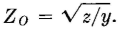
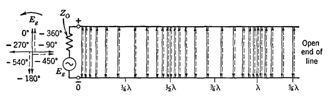
Voltage Distribution on an Open-Circuited Lossless LineFigure 5 shows a generator of open-circuit voltage Eg and internal impedance Zg = Z0 connected to a line that is five-fourths wavelength long; that is, V/f = λ, and l/λ = 5/4, where l is the line length. The condition shown in Fig. 5 is at the instant that the generated alternating signal voltage Eg is a maximum positive value. At this instant, the distribution of the electric field and the initial voltage wave along the line are as shown by the solid arrows. Because of the finite velocity of propagation, at a distance 1/2λ from the sending
end, and at the instant under consideration, the initial voltage wave traveling toward the distant end will be directed as indicated. Since λ/2 equals 180°, the initial wave component at a distance λ/2 from the sending end is equal and opposite to the initial wave component at the sending end. This component was created by the voltage when the impressed voltage was at the position -180°. At a distance A from the sending end the initial voltage wave component will be directed downward, because it represents an impulse sent into the line when the impressed signal voltage was at the position marked -360°.
It will be noted that at the instant under consideration (when the impressed voltage is a maximum positive value) the initial impulse arriving at the distant end is zero. This is because the voltage at -450° (5/4*λ = 450°) was passing through zero. The reflected wave component at point A on the line has traveled a distance 5/4*λ or 450° from the generator to the end of the line, was reflected at the end of the line, and has traveled back λ/4 or 90° to point A. This reflected wave component (shown by broken arrows) was created at -540° as shown by the broken arrow at -540°. The preceding discussion assumes that the voltage wave is reflected at the open-circuited end of the line without a change in phase. This is true, because electric lines of force are assumed to extend from a positive wire to a negative wire, and, since there is no conducting path at the distant end, no interchange of charges from wire to wire can occur. The instantaneous directions of action (and not of travel) of the reflected-voltage component and the initial-voltage component are the same, and, for this reason, the electric field and the voltage component of an electromagnetic wave are reflected with no change in phase from an open circuit at the end of a line. The preceding discussion and Fig. 5 considered the voltage distribution at the instant that the impressed voltage was a maximum positive value. This also is considered in Fig. 6(a). Both illustrations indicate that the resultant voltage wave at the instant under consideration is zero at all points along the line. This resultant voltage wave is the sum of the instantaneous initial and reflected waves. The distributions of the initial, reflected, and resultant voltage waves at other positions of the instantaneous applied voltage are also shown in Fig. 6. It will be noted that in Fig. 6 (a) the resultant voltage is zero, that in Fig. 6(b) the initial and reflected waves add directly, that in Fig. 6(c) the resultant again is zero, and that in Fig. 6(d) the waves again add directly. If voltmeters that indicate effective values of voltage (and not instantaneous values) were connected across the line at regular intervals, a plot of the instrument readings (effective values) would be as indicated by Fig. 6(e). Such a plot of voltage is usually referred to as a voltage standing wave or as a stationary wave.1 Neither of these terms is particularly descriptive of the phenomenon. A plot of effective values of voltage, appearing as in Fig. 6(e), is not a wave in the usual sense. However, the term "standing wave" is in widespread use.
|
|||||
| Home Transmission Lines Voltage Distribution on an Open-Circuited Lossless Line |
|
||||

Last Update: 2011-05-30