Computation of Potential Gradients

Author: Edmund A. Laport

Any solution for the potential at a point in space near the conductors of a transmission line can be applied to the computation of the potential gradient at the surface of a conductor. The potential can be computed for a point very near to the conductor and compared with the potential at the surface. The fall in potential from the conductor surface to the point in space, divided by the distance between them, will yield an average gradient. The exact solution can be obtained by differentiating the potential equation at the surface of any of the conductors, which would give the rate of change of potential versus distance from the conductor. A practical approximation which is simpler will suffice for engineering usage. If the distance between the surface of a conductor and a point in space at which the potential is computed is very small with respect to the radius of the conductor, the potential difference across this space divided by the distance will give a gradient that can be converted to standard units, such as volts per inch or volts percent.meter. For example, if we compute the potential on a wire of a system of radius ρ₁, and then compute the potential at a point distant Δρ, where Δρ is very small with respect to ρ₁, the gradient across Δρ will be very nearly the maximum gradient. If the wire radius is 0.100 inch and we take the point in space 0.005 inch from the surface, the potential at the point would be the same as if the wire was increased in radius by 0.005 to become 0.105 inch, with the same charge on the wire.

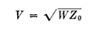
One is usually interested to know the gradient near the high-potential wires of a feeder when a power W is being transmitted into the feeder that is correctly terminated in its characteristic impedance. Then

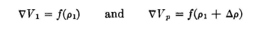
Then, since the potential gradient [#nabla#]V = f( ρ) for a given configuration of wires,

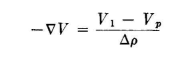
Then the approximate potential gradient [#nabla#]V will be

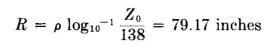
This is applied to practical design problems as follows: Assume that it is desired to find the approximate potential gradient at the surface of a cylindrical wire of radius 0.100 inch when its potential with respect to ground is 10,000 volts. The wire is far removed from all other wires so that its peripheral-charge distribution is uniform and its electric field strictly radial.

We can employ the device of assuming that this wire is the inner conductor of a coaxial transmission line of very high characteristic impedance - say 400 ohms arbitrarily. For such a value the radius R of the outer conductor must be (from the characteristic-impedance formula for the coaxial line)

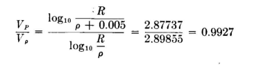
and the ratio R/ ρ = 791.7.

If now we increase ρ by 0.005 inch, so that we can compute the potential at a point 0.005 inch from the wire, and apply the equation previously derived for the potential at a point in the dielectric space of a coaxial line, we obtain, by using five-place logarithms,

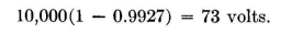
The fall in potential across the first 0.005 inch from the wire is

The average gradient across this distance is then 73/0.005 = 14,600 volts per inch.

The same method can be applied to determine the potential gradient at the surface of the high-potential wires of any transmission line for which the characteristic-impedance formula is known. The reason for this is that when the charge per unit length remains constant, the potential of a wire decreases as its periphery increases, or, as a consequence, as its characteristic impedance decreases. Since the accuracy of the results depends upon the accuracy of very small differences, slide-rule accuracy is not sufficient and the computations should be carried out to four or, preferably, five significant decimal places.