| Electrical Communication is a free textbook on the basics of communication technology. See the editorial for more information.... |

|
Home  Transmission Lines Derivation of Transmission Equations Transmission Lines Derivation of Transmission Equations |
|||


|
  |
||
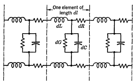
Derivation of Transmission EquationsAn open-ware line (or a cable) is composed of a large number of elements dl, as shown in Fig. 3. If current flows through an impedance, the voltage drop is Iz, and therefore the voltage drop along the element of line dl will be
As a current progresses down the line, a certain amount is lost through parallel admittance y consisting of the shunt conductance and the capacitance of each element. This current loss at each element is Ey, and thus
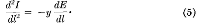
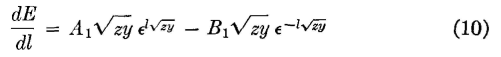
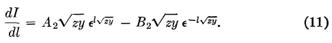
It is now necessary to differentiate these two equations to eliminate E and I. Thus, when equation 2 is differentiated with respect to l it becomes
similarly, equation 3 becomes
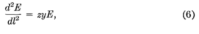
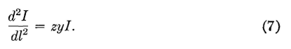
The undesired variables can now be eliminated by substituting in equations 4 and 5 the values from equations 3 and 2 respectively. Then,
and
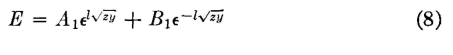
These two equations are simple linear differential equations of the second order, and a knowledge of differential equations is required for their solution. Without presenting the details, the general solution for equations of this form is
and
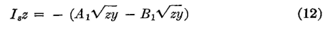
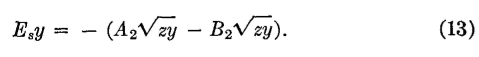
The four constants of integration A1, B1, A2, and B2 must now be found. To do this, equations 8 and 9 are first differentiated with respect to l. They then become
and
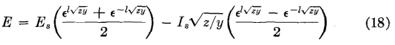
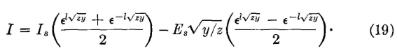
It will be noted that these two expressions are equal to equations 2 and 3, respectively. It can therefore be written that at the sending end, where l = 0,
and
These values are preceded by a negative sign because the current / and the voltage E in any part of the line are less than the sending-end values Is and Es in the infinite line (having no reflection) under consideration. If l is also assumed equal to zero in equations 8 and 9, then E becomes the sending-end voltage Es, and
Similarly,
When these values of A1 and B1 are substituted in equations 12 and 13?
Also,
Furthermore, when these values of A1, B1, A2, and B2 are substituted in equations 8 and 9,
and
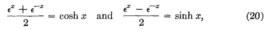
Although it would be possible to use these equations in this form; they can be simplified by the use of hyperbolic functions. In textbooks on this subject it is shown that
where cosh x and sinh x are the hyperbolic cosine and sine, respectively. Accordingly, equations 18 and 19 become
and
These two equations give the voltage E or the current I (in either maximum or effective values) at any point l miles from the sending end of a line having a series impedance of z = R-jX (where X = 2πfL) ohms per loop mile, and a parallel admittance of y = G + jB (where B = 2πfC) mhos per loop mile (page 194). If the values in equations 12 and 13 had been preceded by a positive instead of a negative sign and if Er and Ir had been used, equations for voltage and current at any point in the line in terms of the receiving-end voltage and current and the distance l from the receiving end would have been obtained. These equations are
and
Equations 21, 22, 23, and 24 are general transmission equations applying, for steady-state conditions, to telephone lines and cables. Other methods of deriving these equations are also available (references 2 to 7 inclusive).
|
|||
| Home Transmission Lines Derivation of Transmission Equations |
|
||


Last Update: 2011-05-18