Open-Wire Telephone Lines at Audio Frequencies

TABLE III

CHARACTERISTICS OF EXCHANGE OPEN-WIRE LINES

The use of Table IV and the equations of the preceding section will now be considered. A non-pole pair side circuit of hard-drawn 165-mil copper wires spaced 12 inches apart will be used as an illustration, the frequency will be 1000 cycles, and the temperature 20°C.

Calculation of Linear Electrical Constants. The series resistance R is found as follows: R_dc = ρl/d² = 10.37 x 2 x 5280/165² = 4.02 ohms per loop mile. For hard-drawn copper the resistance is assumed 3 per cent greater; hence, R_dc = 4.02 X 1.03 = 4.14 ohms per loop mile. From equation 67, x = 0.271 d*sqrt(f) = 0.271 x 165 x sqrt(1000 x 10^-6) = 1.41, and, when this is applied to Fig. 15, it is seen that the skin effect is negligible at 1000 cycles. Table IV gives 4.11 ohms.

The series inductance L is calculated by equation 69. L = 0.64374

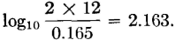
Evaluating the portion

gives

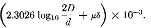
As stated on page 217, μδ = 0.25 for copper at

audio frequencies. Thus, the inductance is L = 0.64374(2.3026 x

CHARACTERISTICS OF STANDARD TYPES OF OPEN-WIRE LONG-DISTANCE TOLL TELEPHONE CIRCUITS COPPER WIRE - 1000 CYCLES PER SECOND

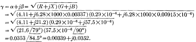
NOTES: 1. All values are for dry weather conditions.

2. All capacitance values assume a line carrying 40 wires.

3. Resistance values are for temperature of 20° C (68° F).

4. DP Insulators assumed for all 12-inch and 18-inch spaced wires-CS Insulators for all 8-inch spaced wire.

5. Open-wire lines are no longer loaded in the United States.

2.163 + 0.25) x 10^-3 = 3.37 x 10^-3 henry, or 0.00337 henry per loop mile, or per mile of line. This agrees with Table IV.

The shunt capacitance C is calculated by equation 70, C = [0.019415/lg(2D/d)] x 10^-6, which for the line under consideration is C = [0.019415/lg(24/0.165)] X 10^-6 = 0.00898 x 10^-6 farad, or 0.00898 microfarad per mile. This is the value of the capacitance in free space and will not agree exactly with Table IV, which is for pairs on a 40-wire line.

The shunt conductance G is not calculated. From Table IV, the value is 0.29 micromho per mile.

Calculation of Propagation Constant. The actual constants from Table IV, instead of the constants just calculated, will be used for subsequent calculations. These are R = 4.11 ohms, L = 0.00337 henry, C = 0.00915 X 10^-6 farad, and G = 0.29 X 10^-6 mho. At 1000 cycles, and from equation 37,

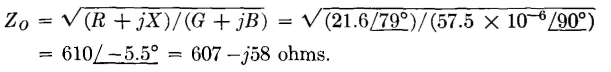
Thus, the attenuation constant a = 0.00339 neper, or 0.00339 X 8.686 = 0.0295 decibel per mile. The phase constant β = 0.0352 radian or 0.0352 X 57.3° = 2.01° per mile. These values agree approximately with Table IV.

Calculation of Characteristic Impedance. From equation 50,

Calculation of Wavelength and Wave Velocity. From equation 54, λ = 2π/β = 6.28/0.0352 = 179 miles; or, λ = 360°/2.01° = 179 miles. From equation 55, V = ω/β = 6.28 x 1000/0.0352 = 179,000 miles per second, or V = λf = 179 x 1000 = 179,000 miles per second.

Calculation of Line Performance. A power input of 0.001 watt, or 1.0 milliwatt, at 1000 cycles is the standard testing power used in checking the performance of telephone lines. Calculations will be made on a section of line 250 miles long, and terminated in 610 ohms pure resistance, a value that simulates the characteristic impedance Z₀ sufficiently close for practical purposes. It will be assumed that the line input impedance also is 610 ohms resistance.

The input voltage will be E = sqrt(PR) = sqrt(0.001 x 610) = 0.782 volt.

The input current will be I = sqrt(P/R) = sqrt(0.001/610) = 0.00128 ampere, or I = E/R = 0.782/610 == 0.00128 ampere.

The received power can be found from equation 49, page 86, P_r = P_s10^-0.1ln = 1.0 x 10^-0.1x7.5 = 0.178 milliwatt, or 0.000178 watt.

The value ln = 7.5 is the loss in decibels for the 250-mile section of line

having a loss of 0.03 decibel per mile from Table IV.

The received voltage can be found from equation 53, E_r = E_s10^-05ln = 0.782 x 10^-0.05x7.5 = 0.33 volt. Or the received voltage is sqrt(0.000178) x 610 = 0.33 volt.

The received current can be found from equation 52, I_r = I_s10^-0.05ln =

0.00128 x l0^-0.05x7.5 = 0.00054 ampere. Or the received current is

0.33/610 = 0.00054 ampere or 0.54 milliampere.

The loss on a typical open-wire line at frequencies higher than 1000

cycles is given in Fig. 18.