| Electrical Communication is a free textbook on the basics of communication technology. See the editorial for more information.... |

|
Home  Radio Wave Propagation and Antennas Ground-Wave Propagation Radio Wave Propagation and Antennas Ground-Wave Propagation |
|||


|
  |
||
Ground-Wave PropagationThe Austin-Cohen formula6 was used until about 1930 to calculate field strengths at a distance from a transmitting antenna. Its use has been largely superseded by the Sommerfeld formula as modified by several investigators.18,19,20,21,22 Of particular interest is the problem of calculating the field strengths produced by standard amplitude-modulation broadcast stations. In engineering practice, curves16 are usually used for this purpose; a summary of the method follows. The field strength produced at a distance by a short vertical antenna (about 0.1λ in length) over perfect earth is23
where E1' is the field strength in millivolts per meter at one kilometer when P is the power input to the antenna in kilowatts. For the field strength at one mile, the equation is23
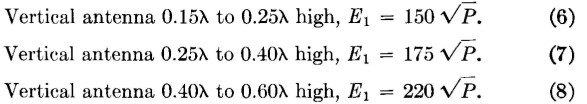
For an actual broadcast-type antenna, different factors16 are used, and the equations are modified23 as follows:
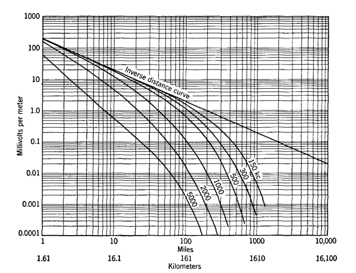
In these three equations, E1 is the field strength in millivolts per meter at one mile and P is the power input to the antenna in kilowatts. The constants for these three equations include such factors as the effect of height and the efficiencies of the antenna and ground system. Note that the field strength is proportional to the square root of the power input. The strength of the ground wave at distances greater than one mile is found from curves. These are available6,16,21,22,23 for various earth conductivities and dielectric constants. In Fig. 9 are included22 curves for good earth conditions, such as encountered in midwestern United States. These curves are based on a field strength of 186 millivolts per meter at one mile and, for a station that does not produce this signal strength, the ordinates of Fig. 9 should be multiplied by the ratio of the actual field at one mile to 186. These curves indicate that ground-wave propagation at high frequencies becomes very inefficient because of losses in the surface of the earth and in objects on the surface. For this reason, high-frequency transmission is not used where ground-wave reception is desired. An inverse-distance curve also is given in Fig. 9. This represents transmission over lossless earth, and the decrease is caused by dispersion, or spreading out of the wave. Signal strengths at a receiving location for good reception are as follows:16 City business or factory areas 10 to 50 millivolts per meter. City residential areas 2 to 10 millivolts per meter. Rural areas 0.1 to 1.0 millivolt per meter. Radio reception is entirely satisfactory under favorable static and noise conditions with weaker signals, perhaps as low as 10 microvolts per meter and even less. Theoretically, 1 millivolt per meter will induce a voltage of 1 millivolt in a wire one meter long if the wire is parallel to the electric lines of force in the received wave. The ground wave from a vertical antenna is not exactly vertically polarized. The losses in the earth cause the wave front to tilt forward slightly.
|
|||
| Home Radio Wave Propagation and Antennas Ground-Wave Propagation |
|
||


Last Update: 2011-05-30