| The ebook Elementary Calculus is based on material originally written by H.J. Keisler. For more information please read the copyright pages. |

|
Home  Integral Theorems of Calculus Theorem 1: Arbitrary Infinitesimals Integral Theorems of Calculus Theorem 1: Arbitrary Infinitesimals |
|


|
  |
Theorem 1: Arbitrary Infinitesimals
THEOREM 1 Given a continuous function f on [a, b] and two positive infinitesimals dx and du, the definite integrals with respect to dx and du are the same,
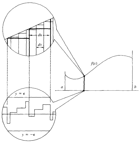
From now on when we write a definite integral that dx is a positive infinitesimal. By Theorem 1, it doesn't matter which infinitesimal. The proof of Theorem 1 is based on the following intuitive idea. Figure 4.2.1 shows the two Riemann sums
Figure 4.2.1 Theorem 1 shows that whenever Δx is positive infinitesimal, the Riemann sum is infinitely close to the definite integral,
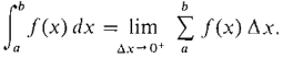
This fact can also be expressed in terms of limits. It shows that the Riemann sum approaches the definite integral as Δx approaches 0 from above, in symbols
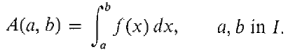
Given a continuous function f on an interval I, Theorem 1 shows that the definite integral is a real function of two variables a and b,
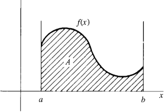
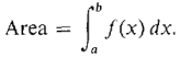
We now formally define the area as the definite integral shown in Figure 4.2.2.
Figure 4.2.2 DEFINITION If f is continuous and f (x) ≥ 0 on [a, b], the area of the region below the curve y = f(x) from a to b is defined as the definite integral:
The next two theorems give basic properties of the integral.
|
|
| Home Integral Theorems of Calculus Theorem 1: Arbitrary Infinitesimals |
|

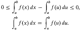
 , it is understood
 and
and  . We see from the figure that the difference
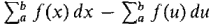 is a sum of rectangles of infinitesimal height. These difference rectangles all lie between the horizontal lines y = -ε and y = ε, where ε is the largest height. Thus


Last Update: 2010-11-26