| The ebook FEEE - Fundamentals of Electrical Engineering and Electronics is based on material originally written by T.R. Kuphaldt and various co-authors. For more information please read the copyright pages. |

|
Home  Reference Algebra Reference Reference Algebra Reference |
|


|
  |
|
Algebra ReferenceAlgebraic identities 
Note: while division by zero is popularly thought to be equal to infinity, this is not technically true. In some practical applications it may be helpful to think the result of such a fraction approaching infinity as the denominator approaches zero (imagine calculating current I=E/R in a circuit with resistance approaching zero -- current would approach infinity), but the actual fraction of anything divided by zero is undefined in the scope of "real" numbers. Properties, arithmetic The associative propertyIn addition and multiplication, terms may be arbitrarily associated with each other through the use of parentheses: 
The commutative propertyIn addition and multiplication, terms may be arbitrarily interchanged, or commutated: 
The distributive property
Properties, exponents 
Properties, radicals Definition of a radicalWhen people talk of a "square root," they're referring to a radical with a root of 2. This is mathematically equivalent to a number raised to the power of 1/2. This equivalence is useful to know when using a calculator to determine a strange root. Suppose for example you needed to find the fourth root of a number, but your calculator lacks a "4th root" button or function. If it has a yx function (which any scientific calculator should have), you can find the fourth root by raising that number to the 1/4 power, or x0.25. 
It is important to remember that when solving for an even root (square root, fourth root, etc.) of any number, there are two valid answers. For example, most people know that the square root of nine is three, but negative three is also a valid answer, since (-3)2 = 9 just as 32 = 9. Properties of radicals
Constants, mathematical Euler's numberEuler's constant is an important value for exponential functions, especially scientific applications involving decay (such as the decay of a radioactive substance). It is especially important in calculus due to its uniquely self-similar properties of integration and differentiation. e approximately equals: 2.71828 18284 59045 23536 02874 71352 66249 77572 47093 69996 
PiPi (π) is defined as the ratio of a circle's circumference to its diameter. Pi approximately equals: 3.14159 26535 89793 23846 26433 83279 50288 41971 69399 37511
Note: For both Euler's constant (e) and pi (π), the spaces shown between each set of five digits have no mathematical significance. They are placed there just to make it easier for your eyes to "piece" the number into five-digit groups when manually copying. Definition of a logarithmLogarithm
"log" denotes a common logarithm (base = 10), while "ln" denotes a natural logarithm (base = e). Properties of logarithms Transform function, definition of
These properties of logarithms come in handy for performing complex multiplication and division operations. They are an example of something called a transform function, whereby one type of mathematical operation is transformed into another type of mathematical operation that is simpler to solve. Using a table of logarithm figures, one can multiply or divide numbers by adding or subtracting their logarithms, respectively. then looking up that logarithm figure in the table and seeing what the final product or quotient is. Slide ruleSlide rules work on this principle of logarithms by performing multiplication and division through addition and subtraction of distances on the slide. 
Marks on a slide rule's scales are spaced in a logarithmic fashion, so that a linear positioning of the scale or cursor results in a nonlinear indication as read on the scale(s). Adding or subtracting lengths on these logarithmic scales results in an indication equivalent to the product or quotient, respectively, of those lengths. Most slide rules were also equipped with special scales for trigonometric functions, powers, roots, and other useful arithmetic functions. Factoring 
Quadratic formula 
Sequences Arithmetic sequence Common difference Difference, common Arithmetic sequencesAn arithmetic sequence is a series of numbers obtained by adding (or subtracting) the same value with each step. A child's counting sequence (1, 2, 3, 4, . . .) is a simple arithmetic sequence, where the common difference is 1: that is, each adjacent number in the sequence differs by a value of one. An arithmetic sequence counting only even numbers (2, 4, 6, 8, . . .) or only odd numbers (1, 3, 5, 7, 9, . . .) would have a common difference of 2. In the standard notation of sequences, a lower-case letter "a" represents an element (a single number) in the sequence. The term "an" refers to the element at the nth step in the sequence. For example, "a3" in an even-counting (common difference = 2) arithmetic sequence starting at 2 would be the number 6, "a" representing 4 and "a1" representing the starting point of the sequence (given in this example as 2). A capital letter "A" represents the sum of an arithmetic sequence. For instance, in the same even-counting sequence starting at 2, A4 is equal to the sum of all elements from a1 through a4, which of course would be 2 + 4 + 6 + 8, or 20. 
Geometric sequencesGeometric sequence Common ratio Ratio, commonA geometric sequence, on the other hand, is a series of numbers obtained by multiplying (or dividing) by the same value with each step. A binary place-weight sequence (1, 2, 4, 8, 16, 32, 64, . . .) is a simple geometric sequence, where the common ratio is 2: that is, each adjacent number in the sequence differs by a factor of two. 
Factorial ! (factorial) Definition of a factorialDenoted by the symbol "!" after an integer; the product of that integer and all integers in descent to 1. Example of a factorial: 
Strange factorials
Simultaneous equations Systems of linear equations The terms simultaneous equations and systems of equations refer to conditions where two or more unknown variables are related to each other through an equal number of equations. Consider the following example: 
For this set of equations, there is but a single combination of values for 
Each line is actually a continuum of points representing possible Usually, though, graphing is not a very efficient way to determine the simultaneous solution set for two or more equations. It is especially impractical for systems of three or more variables. In a three-variable system, for example, the solution would be found by the point intersection of three planes in a three-dimensional coordinate space -- not an easy scenario to visualize. Substitution methodSubstitution method, simultaneous equationsSeveral algebraic techniques exist to solve simultaneous equations. Perhaps the easiest to comprehend is the substitution method. Take, for instance, our two-variable example problem:
In the substitution method, we manipulate one of the equations such that one variable is defined in terms of the other: 
Then, we take this new definition of one variable and substitute it for the same variable in the other equation. In this case, we take the definition of 
Now that we have an equation with just a single variable ( 
Now that 
Applying the substitution method to systems of three or more variables involves a similar pattern, only with more work involved. This is generally true for any method of solution: the number of steps required for obtaining solutions increases rapidly with each additional variable in the system. To solve for three unknown variables, we need at least three equations. Consider this example: 
Being that the first equation has the simplest coefficients (1, -1, and 1, for 
Now, we can substitute this definition of 
Reducing these two equations to their simplest forms: 
So far, our efforts have reduced the system from three variables in three equations to two variables in two equations. Now, we can apply the substitution technique again to the two equations 
Next, we'll substitute this definition of 
Now that 
Now, with values for 
In closing, we've found values for Addition methodAddition method, simultaneous equationsWhile the substitution method may be the easiest to grasp on a conceptual level, there are other methods of solution available to us. One such method is the so-called addition method, whereby equations are added to one another for the purpose of canceling variable terms. Let's take our two-variable system used to demonstrate the substitution method:
One of the most-used rules of algebra is that you may perform any arithmetic operation you wish to an equation so long as you do it equally to both sides. With reference to addition, this means we may add any quantity we wish to both sides of an equation -- so long as it's the same quantity -- without altering the truth of the equation.
An option we have, then, is to add the corresponding sides of the equations together to form a new equation. Since each equation is an expression of equality (the same quantity on either side of the 
Because the top equation happened to contain a positive 
Once we have a known value for 
We could add these two equations together -- this being a completely valid algebraic operation -- but it would not profit us in the goal of obtaining values for 
The resulting equation still contains two unknown variables, just like the original equations do, and so we're no further along in obtaining a solution. However, what if we could manipulate one of the equations so as to have a negative term that would cancel the respective term in the other equation when added? Then, the system would reduce to a single equation with a single unknown variable just as with the last (fortuitous) example.
If we could only turn the 
Now, we may add this new equation to the original, upper equation: 
Solving for 
Substituting this new-found value for 
Using this solution technique on a three-variable system is a bit more complex. As with substitution, you must use this technique to reduce the three-equation system of three variables down to two equations with two variables, then apply it again to obtain a single equation with one unknown variable. To demonstrate, I'll use the three-variable equation system from the substitution section:
Being that the top equation has coefficient values of 
We can rid the bottom equation of its 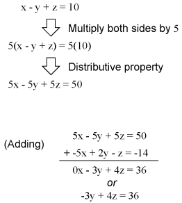
At this point, we have two equations with the same two unknown variables, 
By inspection, it should be evident that the 
Taking the new equation Contributors to this chapter are listed in chronological order of their contributions, from most recent to first. See Appendix 2 (Contributor List) for dates and contact information. Chirvasuta Constantin (April 2, 2003): Pointed out error in quadratic equation formula.
|
|
| Home Reference Algebra Reference |
|
Last Update: 2010-12-01