| Electrical Engineering is a free introductory textbook to the basics of electrical engineering. See the editorial for more information.... |
|
Home  Commercial Forms of EMF, Power and Energy Instantaneous Values of Electromotive Force Commercial Forms of EMF, Power and Energy Instantaneous Values of Electromotive Force |
|||||||||
| See also: Electromotive Force Produced by Motion | |||||||||


|
  |
||||||||
|
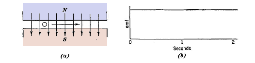
Instantaneous Values of Electromotive ForceAuthor: E.E. Kimberly When a conductor moves with uniform velocity through a magnetic field of uniform intensity, there is generated in that conductor an emf of constant value. See Fig. 2-1 (b). This is called direct emf.1 If, however, the field is not of uniform intensity, or for any other reason the rate of cutting flux lines is not constant, then the emf generated is not of constant value.
Assume that in Fig. 2-2 (a) the flux in the airgap between the poles N and S is of uniform intensity and that the angular velocity of the conductor shown is 2π radians per second and is constant. Fig. 2-2 (b) is a plot of the rate at which the conductor cuts the magnetic field at every point in one revolution. The generated emf wave is, hence, of the same shape. In position A, Fig. 2-2 (a), the motion of the conductor is parallel to the lines of flux of the field; and, since no flux is being cut, no emf is being generated. This instant of time corresponds to A in Fig. 2-2 (b). In position C in (a) the conductor is moving at right angles to the lines of flux, and hence the rate of cutting these lines is maximum. This position corresponds to the instant C in Fig. 2-2 (b). Between positions A and C the rate of cutting the magnetic field is a sinusoidal function of position and, therefore, of time. After position E is reached, the conductor begins to cut across the field in the opposite direction, and hence its generated emf is reversed in direction and is shown as negative on the sinusoid. In making one complete revolution in 1 second, the conductor has generated in it all possible values of emf at a fixed speed and with a fixed flux intensity; hence, the emf is said to have completed one cycle. The number of cycles completed in 1 second is called the frequency. Thus, the emf in Fig. 2-2 has a frequency of 1 cycle per second. The instantaneous value of a sinusoidal emf is frequently expressed as e = Em sin ωt (2-1) where e = instantaneous value of the emf; On the North American continent 25-cycle, 40-cycle, 50-cycle, and 60-cycle frequencies only are in commercial power use. Current caused to flow in a circuit by sinusoidally varying voltage is called alternating current.
If the magnetic field of Fig. 2-2 (a) were not of uniform intensity, the emf generated would, of course, be alternating, but would not be sinusoidal. In many cases in practical engineering the generated electromotive forces and currents are not sinusoidal. In almost all modern alternating-current generators the conductors are stationary and the magnetic poles are rotated past them at constant speed. However, the fluxes from the poles cannot effectively be distributed over the pole faces so as to produce a sinusoidal voltage under all conditions of loading. The voltage produced by any particular coil of the generator looks approximately like that shown in Fig. 10-5 (a). However, by using many coils and shaping them properly, the terminal voltage wave shape is made so nearly sinusoidal that it may be considered as such for practically all purposes.
|
|||||||||
| Home Commercial Forms of EMF, Power and Energy Instantaneous Values of Electromotive Force |
|
||||||||