Radiation Characteristics of a Vertical Radiator

Author: Edmund A. Laport

The type of radiator that is generally used for medium-frequency broadcasting is the straight uniform vertical with its lower end near ground. This type is also used for certain limited applications at the higher frequencies, and to some extent at lower frequencies. Such antennas may be steel towers used as radiators or supported vertical wire antennas. Extensive experience has been gained with vertical radiators at many hundreds of broadcast stations, each employing one or more for omnidirectional or directive radiation.

The radiation pattern for a vertical radiator is uniform in the horizontal plane (nondirective) but is directive in the vertical plane. The vertical directivity pattern depends on the distribution of currents in the radiator. If the radiator is of uniform cross section throughout its length, the current distribution is virtually sinusoidal; that is, the amplitude of the current is a sinusoidal function of the electrical distance from its upper end. This approximation does not lead to very serious deviations from physical fact for ordinary engineering purposes, and the simplifications in computations are desirable.

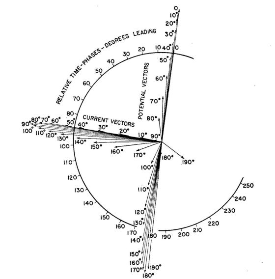
Pure sinusoidal distribution is the consequence of a pure standing wave on the radiator, which means that there are no losses whatever in the system. In fact, energy loss due to radiation and circuital loss requires that the actual current distribution be composed of a standing wave and a smaller component of traveling wave, the latter supplying the actual losses. In measurements that have been made of current distributions, the effect of the feed current due to the traveling-wave component is conspicuous only in the region of a current node, where instead of the current becoming zero, as it would from a pure sinusoidal distribution, it passes through a minimum value. At this minimum, the current has changed phase by 90 degrees and is then in phase with the antenna potential. The impedance therefore appears as a pure resistance at this point.

It is very helpful to the antenna engineer to have a clear physical concept of the manner in which waves are propagated in a linear conductor such as a vertical radiator and how the potentials, currents, and antenna impedance vary with its electrical length. For engineering purposes, the concept is sufficiently exact if the antenna is treated as an open-ended transmission line of uniform characteristic impedance.

In Figs. 2.4A and 2.4B there is represented graphically the solution of the current and potential distributions and the vector relations between potential and current at all points along a vertical radiator 190 degrees high.

Figure 2.4A represents an attenuated traveling wave propagated in the antenna when excited by a generator connected between its base and ground.

FIG. 2.4A. Development of current and potential distributions on a uniform vertical radiator 190 degrees high, representing the attenuation of a transmitted and reflected wave of charges, when the radiator is fed between its base and ground.

For the time it takes to propagate this wave from the generator to the top of the antenna,and back, the antenna appears to the generator as a resistance equal to its characteristic impedance. Therefore the potential and current vectors of the upward wave and the downward wave of charges are in phase. The envelope of these vectors of the traveling wave that goes up and down the antenna is a logarithmic spiral.

Owing to the complete reflection of this traveling wave from the open end of the antenna, the vector sum of the currents from the upward and

FIG. 2.4B. Development of current and potential distributions on a uniform vertical radiator 190 degrees high, representing the attenuation of a transmitted and reflected wave of charges, when the radiator is fed between its base and ground.

the downward waves must cancel to zero at the open end. This is accomplished by a reversal of the current vector in the downward wave. The potential vectors at the top add to double the potential of the traveling wave at that point.

The potential (and current) at any point in the antenna are the vector sums of the potentials (and currents) at that point due to the upward wave and the downward wave with their propagation time-phase differences from that point to the top end and back again. This effect is illustrated for the point 70 degrees from the upper end in Fig. 2.4A, where the resultant potential at that point is shown to be obtained by adding the potential vectors for the two traveling waves and the resultant current by subtracting the current vectors. It is seen that at this point the resultant current vector leads the resultant potential vector by an angle 0 less than 90 degrees. The antenna impedance at this point looking toward the open end is therefore R - jX.

Figure 2.4B is a polar plot of the resultants of performing similar vector additions of the potential vectors and vector subtractions of the current vectors at 10-degree intervals along the entire 190-degree antenna. These relations are more accurately tabulated in Table 2.4. Since in this diagram we are using the electrical distance from the top of the antenna, the 190-degree point is at the base near ground where the system is usually fed.

Therefore the vector ratio V₁₉₀/I₁₉₀ represents the input impedance of the antenna between ground and its lower end. This of course omits consideration of any additional stray capacitance in parallel with this impedance which would be introduced by the physical construction of an actual antenna.

When the resultant potential and current vectors of Fig. 2.4B are plotted as in Fig. 2.5, we see the potential and current distributions in the manner most frequently displayed and described. In this diagram, only the magnitudes are shown, whereas in Fig. 2.4B both magnitude and phase are shown. The comparison with sinusoidal theory is indicated also.

From Fig. 2.4B it can be seen how the impedance looking toward the upper end from any point varies with the location of the point. It is evident that:

1. At all points less than 90 degrees from the upper end the impedance is R - jX and that R increases and X decreases as the distance from the end increases.

2. At the 90-degree point, the impedance is pure resistance, and the resultant potential vector has turned 90 degrees from the open end.

3. Between 90 degrees and 180 degrees the potential vector leads the current vector so that the impedance looking upward from any of these points is R + jX, with resistance and reactance both increasing with increased distance from the top.

4. At the 180-degree point the current is in phase with the potential, and their ratio is such as to give an impedance that is a high value of resistance. Therefore the reactance had to change from a high value at some point less than 180 degrees to fall rapidly to zero at the 180-degree point.

5. Beyond the 180-degree point we see the beginning of another cycle of events where the potential is falling, the current is rising, and the current is leading the potential. It is evident, therefore, that between 180 degrees and 270 degrees the antenna impedance would be R - jX again, but with both R and X decreasing with increase of length.

6. All these cycles of changing sign of reactance and changing values of resistance and reactance are typical of an open-circuited transmission line with attenuation. Qualitatively the analogy is satisfactory. Quantitatively the analogy fails to provide sufficient accuracy so that empirical data like that of Figs. 2.15 and 2.16 have to be used for engineering-design purposes.

FIG. 2.5. Comparison of current distributions for sine and actual relative values on a 190-degree uniform vertical radiator.