Lobe-splitting Technique

Author: Edmund A. Laport

Let G(β) be the radiation pattern for a pair of radiators (each radiator havinga circular pattern) with spacing Si in electrical degrees and equal currents of such phase (φ i) as to place a null at an angle of βi each side of the axis. This arrangement is illustrated in Fig. 2.40A. Then

Now consider the case where each radiator is replaced by the center of a pair of radiators having the pattern H( β) with axis coincident with

that of G(β), as shown in Fig. 2.40B. Then H( β) is specified by spacing S₂ and phase difference φ₂ so that

This pattern is such as to produce a null at an angle ± β₂ from the array axis. Then, the pattern for an array of two pairs along a common axis with equal currents is

and it will have nulls at ± βi and ± β₂ from the array axis.

This method of using two pairs is sure to provide at least two nulls on each side of the axis, which can be placed as desired. In the case where S₁ = S₂, radiators 2 and 3 become coincident, and the effect of two pairs is achieved with three radiators. The current in the middle radiator must be the vector sum of those for radiators 2 and 3 considered separately.

This process can be continued in further similar steps as desired. The following is given to illustrate a case where this operation has been performed three times.

Example. Wanted a radiating system providing suppression of radiation over an angle of at least 90 degrees on one side, of the pattern, the field strength within this angle to be less than 3 percent of the maximum field from the array (±45 degrees from the axis). Using the principles outlined, let us arbitrarily begin with a basic pair that has nulls at ±43 degrees from the axis of the array, using 180 degrees spacing between radiators. Such a pattern is obtained when φ1 = 48 degrees.

The pattern for this pair is shown by curve A in Fig. 2.41. Let us now use this pair as a directive source for a second pair, using the same spacing, but adjusting the phase to bring nulls at ±30 degrees. The fundamental pair of circular sources gives

This pattern is plotted as curve B in Fig. 2.41.

If at this stage we synthesize the composite pattern

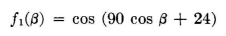
we obtain nulls at ±30 degrees and ±43 degrees. This is plotted as curve C in Fig. 2.41. It is seen that insufficient suppression occurs between 0 and ±30 degrees.

Another pair of radiators spaced 180 degrees and having φ = 8 degrees may be added. This pair will produce a null at β = ±19 degrees. Again

FIG. 2.41. Plots of successive development of broad null region by placing the zeros in successive pairings.

using circular-radiation sources, the radiation pattern (Fig. 2.41, curve D) is

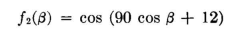
If now this pair is made up of a pair of systems having the pattern f₃(β)f₂(β), we obtain

This is plotted as curve E in Fig. 2.41. The radiation is less than 3 percent of maximum over a range of ±52 degrees. Throughout most of this angle (± 40 degrees) the field strengths are actually less than 1 percent of maximum. This is desirable, because some operating margin is almost always desirable for arrays of this sort.

Array Synthesis. It remains to determine the actual array which will produce this pattern. This is accomplished by the three steps illustrated in Fig. 2.42A, B, and C.

FIG. 2.42. Synthesis of array current distributions for system of Fig. 2.41.

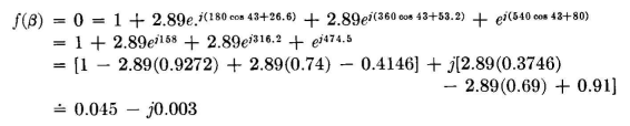
To check the correctness of the foregoing synthesis, the vector method can be applied in the following manner; for the azimuth = ±43 degrees, the location of one of the nulls

The real and imaginary parts equate to very nearly zero by omitting the use of some of the fractions of degrees in obtaining the sines and cosines. This is a satisfactory check on the synthesis process. This vector check provides some idea of the stability required to maintain the pattern. By changing the coefficients corresponding to current amplitudes by small increments the effect on the field in the null regions is quickly found.