Circuital Design

Author: Edmund A. Laport

The desired information for the electrical design of this type of antenna is the following:

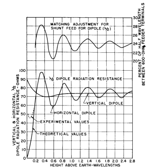
Length of the antenna conductor and its cross-sectional size

Feed-point impedance (depending upon series or shunt feed)

Potential at the ends (for insulator-selection purposes)

Maximum potential gradient for the power to be used

Antenna current at the middle of the dipole

Method of feeding

Efficiency of antenna and feeder system

It is assumed that the height of the dipole has been determined previously from considerations of its radiation-pattern requirements. The height influences the antenna feed-point impedance as shown in Fig. 3.18.

The tolerance on the antenna length is quite liberal if it is to be series-fed at the center, though the radiation resistance will change with length. The length can be of the order of one-half wavelength, and one can omit considerations of end effect of the wire and the insulator hardware. The reason for this is that a 5 percent variation in length makes very little difference in the radiation pattern. The changes in the feed-point impedance are quite immaterial when impedance-matching techniques are applied to terminate the feeder at some point near the antenna, which is usually required.

With shunt feed, as in Fig. 3.19 (if one wishes to use a chart such as that given in the upper portion of Fig. 3.18 for impedance matching) the length of the antenna should be more precise and should be one-half wavelength long, less about 5 percent for end effects. The end effects and the capacitances of strain insulators have the effect of increasing the length of the antenna.

In a typical application one uses a conductor about one-half wavelength long and attaches it to the suspension rigging with the type of insulator suited to the electrical and mechanical duty.

For low-power applications the conductor size will be determined only by the mechanical considerations. However, for medium-power inputs some thought must be devoted to the potential gradients, especially at high altitudes. The larger the conductor diameter, the lower the potential gradients for the same power input and the less possibility of pluming.

FIG. 3.18. Radiation resistance of horizontal and vertical half-wave dipole antennas. (After Carter)

The calculation of the potential gradients at the high-potential points near the ends of the antenna is dependent upon the power input (on modulation peaks for amplitude-modulated services), the height of the antenna above ground, and the wire diameter. The height affects the radiation resistance as shown in Fig. 3.18, and therefore the antenna current and the antenna potential.

A typical example of the procedure by which these important potential details may be calculated is the following.

Example of Computation of Antenna Operating Potential. A 5,000-watt amplitude-modulated transmitter for an aviation communication application on 5,800 kilocycles requires a horizontal half-wave dipole antenna located three-eighths wavelength above ground. The altitude is 4,000 feet. What antenna dimensions must be used, and what potentials will be encountered?

One-half wavelength at 5,800 kilocycles is 86 feet. With end effect and insulator capacitance considered, we can reduce this about 5 percent to 81 or 82 feet. The only important reason for doing so is to decrease tower spacing, which is usually desirable for minimizing mechanical loads and the land area required. The end effects make the system appear electrically as a full half-wavelength, and the current and potential distributions can be considered on that basis.

FIG. 3.19. Horizontal dipole antenna with shunt feed.

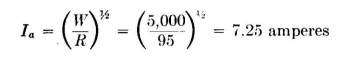
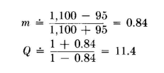
From Fig. 3.18, we read a radiation resistance of 95 ohms at the center of the antenna wire, for a height of three-eighths wavelength (64 feet). For 5,000 watts input on carrier, the antenna current will be

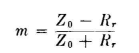
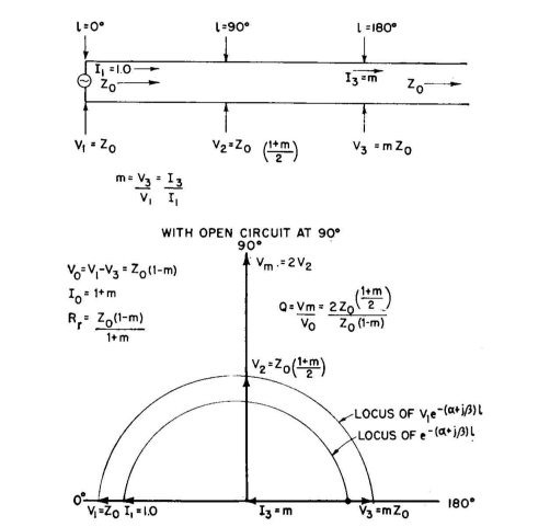
The current is distributed sinusoidally from the virtual end, that is, from a point which is extended about 5 percent of length beyond the physical ends of the wire. Maximum current occurs at the center of the antenna. As measured from the end, the potential distribution is very nearly cosinusoidal, except near the center, where it departs considerably from this form. This departure lies in a region about 10 degrees each side of center. Beyond these points, the cosinusoidal distribution can be assumed. Therefore, we know the shape of the distribution but not its numerical magnitude. A simple method is now needed to establish this magnitude within limits that are acceptable for engineering purposes. If we can determine the standing-wave ratio Q for the antenna, the voltage to ground at the end of the dipole V_m will be QV_a/2, where V_a is the balanced voltage applied at the central feed point. V_a = I_aZ_a, the antenna current at the feed point times the feed-point impedance.

The Q of a half-wave dipole can be determined approximately from transmission-line theory by considering an open-ended line of characteristic impedance Z₀ having a length of 90 degrees. This is the same as studying relations of voltages and currents in the first one-half wavelength (180 degrees) of an infinite line with attenuation, because when the line is open-circuited at 90 degrees, the reflected wave will be the same as that between 90 and 180 degrees on the infinite line (see also Sec. 2.3). By combining the direct wave and the reflected wave from the open circuit, the potential and current distributions can be obtained, and the standing-wave ratio. It will be assumed now that the half-wave dipole has a length such that, with its end effects, Z_a = R_a + j0. If the system losses are due entirely to radiation, R_a = Rτ, the radiation resistance, which can be read from Fig. 3.18 as a function of the height of the horizontal dipole from ground.

Applying this method, we first obtain a factor m which is the ratio of the attenuated voltage 180 degrees from the generator on the infinite line to the generator voltage. This is found to be

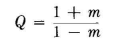
and

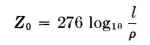
Reference to Fig. 3.20 will clarify the derivation of these equations. The dipole antenna, as a balanced transmission line, has a characteristic impedance

where l is the total length of the dipole in the same linear units as used for its radius ρ.

For low-power and receiving applications the conductor size for the dipole is chosen for its mechanical requirements only. In this example, it is desirable to see that the maximum antenna potential is below the critical corona potential for the altitude and temperature of the site, to ensure safe operation. To do this, we first choose a preferred arbitrary wire size and compute the potential that would exist at rated power input. Then the maximum safe operating potential is computed. The ratio of the latter to the former is the safety factor and is greater than 1.0.

FIG. 3.20. Geometry for computing the approximate Q of the dipole.

Assume that we select a wire for the antenna with a radius of 0.102 inch. Then

The balanced antenna driving voltage V_a = I_aR_a = 7.25 · = 690 volts root-mean-square unmodulated

The potential from one end of the dipole to ground is then

To allow for 100 percent positive modulation, this value must be doubled, to 7,900 volts root-mean-square. This is the working potential for the strain insulators that will support the dipole.