Suppressing Secondary Lobes by Splitting

Author: Edmund A. Laport

It is possible to suppress side lobes in a broadside pattern from a linear arrangement of horizontal dipoles by using successive pair combinations that split the side lobes resulting from the geometry of the original pair. In this method, the currents in all the dipoles are equal and cophased. The side-lobe suppression is obtained entirely by the geometrical spacings of the dipoles.

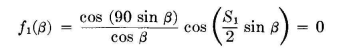
Let it be desired to produce a broadside beam that has its first nulls at plus and minus 15 degrees from the main beam, with all side lobes less than 0.1 in strength compared with the main beam.

The equation for a pair of horizontal dipoles that produces first nulls at plus and minus 15 degrees is

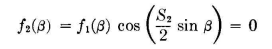
Spacing S₁ is found to be 700 degrees. This spacing also gives a second pair of nulls at plus and minus 51 degrees.

It is evident that a large secondary lobe exists between 15 and 51 degrees, and because this is a rather large angular interval, and because we desire a considerable degree of suppression, we can now replace each of these dipoles with a pair of dipoles spaced a distance S₂ between centers such that we bring a null at 27 degrees. The equation for the linear combination is now

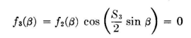
From the last factor, S₂ is computed to be 400 degrees. This pair has but one null. Our nulls are now at 15, 27, 51, and 90 degrees, the null at 90 degrees resulting from the dipole factor. It can be assumed that side lobes will exist about halfway between these nulls.

The angular space between 27 and 51 degrees is a large one, and a large side lobe must exist between these nulls. Thus we can pair the radiators again and get

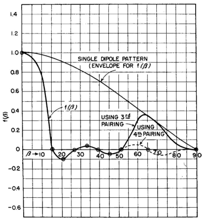
A value for S₃ is now computed that will bring a null at the middle of this side lobe, at about 39 degrees. The center spacing of a pair of dipoles that will achieve this is when S₃ is 290 degrees.

At this stage there are nulls in the patterns at 15, 27, 39, 51, and 90 degrees, and maximums exist at 0, 21, 33, and 45 degrees; and, due to the diminishing value of the dipole factor at the large azimuth angles, we estimate the last lobe at perhaps 65 degrees.

We can now make a quick calculation of the values of the pattern at these angles corresponding to side-lobe maximums to see how we are progressing. We find the following values from the equation above:

0 1.00

21 -0.101

33 0.047

45 -0.048

65 0.345

The desired degree of suppression is obtained in all side lobes except the last. This one can be split up by pairing the radiators in another

Fig. 3.57 :

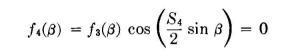
step, obtaining the pattern equation

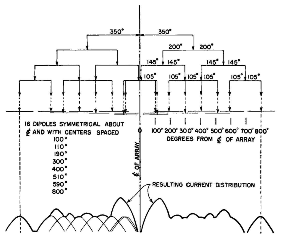
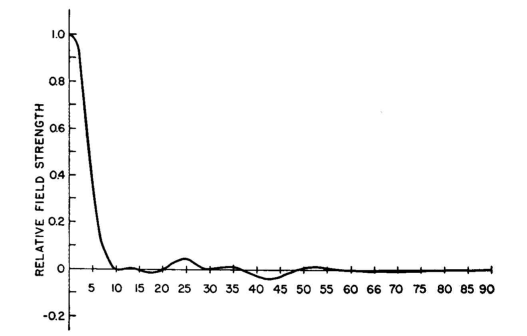
The value of S₄ that will bring a null at 65 degrees is 210 degrees. Without further computation we can plot the known points and, with acceptable accuracy for exploratory purposes, sketch in the pattern between these points, as is done in Fig. 3.57. From this we are certain that the specification has been met in principle.

It now remains to synthesize the final arrangement of the dipoles in this linear array. This process is indicated in Fig. 3.58. The resulting arrangement is complicated because we find that the radiators in the successive pairing operations overlap to a considerable extent.

FIG. 3.58. Synthesis of current distribution that gives the horizontal pattern of Fig. 3.57.

Nevertheless, the realization of such a current distribution by this arrangement of dipoles will actually produce the desired pattern. This particular example was chosen at random to describe the application of a useful principle, but the attainment of such an array is not necessarily practical. Greater practicality of application can be assured in this method if the pair spacings are confined to integral multiples of half wavelengths. Then all the overlapping dipoles will be exactly superimposed in the synthesizing process. It is worth while to test this principle with another example.

Let it be desired to produce a broadside pattern that has its zero at about 10 degrees, and let all secondary lobes be suppressed as much as possible by using the half-wave spacing technique. Following the same procedure as in the preceding example, it is found that the first pair, with a spacing of 1,080 degrees (six half wavelengths) will give nulls at 9.5, 29, and 57.5 degrees. The next pair with five half wavelengths spacing will give nulls at 11.5 and 37 degrees. The third step with four half wavelengths spacing gives nulls at 14.5 and 49 degrees. The fifth step places another null at 20 degrees, and in the sixth step, when the pair spacing is one-half wavelength, there is another null at 30 degrees.

FIG. 3.59. Array horizontal pattern.

The major side lobes are split by a total of 10 zeros between 9.5 and 90 degrees. The resulting pattern will have the equation

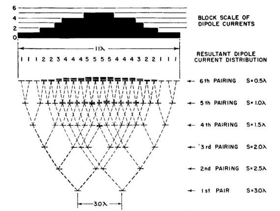
The computation of this pattern is easy with the aid of Appendix V-B, where each pair pattern has already been tabulated. It is necessary only to multiply across the six columns of cophased pairs together with the column for the dipole directivity pattern. The result is shown in Fig. 3.59. The pattern has a half-power beam width of 13 degrees, and none of the side lobes exceed 4.5 percent of the field strength of the main beam. There are two lobes of this intensity, at 25 and 42.5 degrees. All the others are 1 percent or less over the entire range. If a passive reflecting screen were to be used, these would be reduced somewhat more.

The synthesis of the array to give this pattern with half-wave-spaced horizontal dipoles is given in Fig, 3.60. From this we find that the array would require a horizontal width of 22 half-wave dipoles. The loop currents end to end are found to be the following: 1,1,1,2,2,3,4,4,4,5,5,5,5, 4,4,4,3,2,2,1,1,1.

A linear array of this distribution is physically practical to construct and to feed.

The same technique may be applied in the vertical-plane pattern.

FIG. 3.60. Synthesis of current distribution that gives the pattern of Fig. 3.59.