Input Impedance to Any Radiator in an Array of Dipoles

Author: Edmund A. Laport

To excite a radiating system properly, each radiator must have a current of the proper phase and amplitude. Except in the simplest cases, this requires a knowledge of the input impedance of each radiator, clue to its self-impedance Z_kk and the mutual impedance with all other radiators and images of the system. In practice, certain mutual effects can be neglected when it is known that they are of trivial magnitude compared with certain dominant ones. A complete solution, however, must account for the total of all these effects, especially if the currents are to be unequal.

When the elements of an array are half-wave dipoles, prepared data given in Figs. 3.61 and 3.62 may be used for the mutual impedances for parallel and collinear dipoles. Echelon and angular configurations must be computed from basic formulas. Most data of this sort are referred to a current antinode for a half-wave element having sinusoidal current distribution. When half-wave elements are end-fed, the antinode values of impedance must be transformed through one-quarter wavelength of the characteristic impedance of the element used. Such transformations lead to approximations that are of tolerable engineering accuracy.

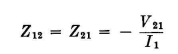
Mutual impedance is defined as the negative ratio of the induced electromotive force at a current antinode in radiator 2 due to the antinode current in radiator 1. By reciprocity, the effects both ways are equal. Thus

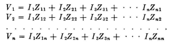
When the values of self- and mutual impedances are known, the system can be computed according to network theory, using the complex form for both currents and impedances. It is emphasized that a vector mutual impedance can lie in any one of four quadrants, and due care must be observed in the computation to account for the most general conditions. When all the currents are equal and cophased, the computations are relatively simple. When the various radiator currents are unequal in amplitude and phase, computations are more complicated.

The equations used to compute the input impedances are as follows: (All V's, I's, and Z's must be in complex (vector) form, indicating magnitude and phase.)

for n radiators numbered in order from 1 to n, having self-impedances Z₁₁, Z₂₂, Z₃₃, etc., and mutual impedances between elements as indicated by the subscripts. Images in the earth and in reflector screens are treated as discreet radiators, taking into account the proper relative directions of currents in corresponding images.

The symmetry characteristic of high-frequency arrays reduces the labor of computation because the computation does not have to be carried out for every radiator in the system. Unsymmetrical arrays require the full treatment.

An element of the system that is parasitically excited from the radiation field of some other element has its potential equated to zero.

The impedance of any radiator k, when properly functioning in the system to give the required radiation pattern, is then the ratio Z_k = V_k/I_k where in general all values are complex. With a knowledge of the feed-point impedance in each radiator of a system, the feeder requirements can be developed for impedance, amplitude, and phase matching of all the currents back to the main power feeder.

Figure 3.18 gives the impedance at the center of a half-wave horizontal dipole, taking into account the mutual impedance with its image, assuming perfectly conducting earth.

If a horizontal dipole is located a distance h degrees above a perfectly conducting earth and a distance d degrees in front of a vertical infinite reflecting plane, there will be inverted images of the dipole a distance h below the surface of the earth and another a distance d behind the reflecting screen. In addition, there will be a third image having the same polarity as the radiator, and located below earth level at the corner of the rectangle 2h·2d formed by the radiator and its two primary images. The impedance of the radiator in this arrangement is

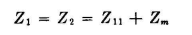
where Z₁₂ is the mutual impedance with the earth primary image, Z₁₃ is the mutual impedance with the screen primary image, and Z₁₄ is the mutual impedance with the earth secondary image.

In all cases where there are two or more primary images there may be one or more secondary images. A radiator located in a corner between intersecting 90-degree planes has two primary images and one secondary image. When the radiator is located between two planes intersecting at 60 degrees, there are two primary images and three secondary images, the polarity of successive images being reversed. For intersecting planes at random angles that are not equal fractions of a circle, there may be an infinity of secondary images. Such cases seldom arise in practice except with the corner-reflector type of system or when a radiator is located between parallel and near-parallel conducting planes. One can study the complex images in such cases with mirrors placed at proper angles, as in a kaleidoscope, using a dot to represent the end of the radiator.

Two identical parallel radiators having equal cophased currents have equal input impedances computed from

In the case of equal antiphased currents,

This condition explains why a radiator parallel to and with very small spacing from a conducting plane has its input impedance greatly reduced by the effect of the relatively large value of Z_m. Thus, for a given power input, the current must be large, and the potentials on the radiator are relatively large as a consequence. Both these factors contribute to increased losses beyond a certain proximity where losses neutralize theoretical gain. This is an example of a general practical fact that high gain in limited space is always attended with limitations due to losses, since all such systems have low input resistance and low radiation resistance. Bandwidth is also reduced in such systems.

Curves of mutual impedance between parallel and collinear half-wave dipoles are given in Figs. 3.61 and 3.62. For formulas for the mutual impedance between dipoles in echelon and at an angle to each other in a common plane, consult Carter , Brown , Kraus , and Terman .

It is seen from Fig. 3.61 that the magnitude of mutual impedance between parallel half-wave dipoles does not fall to one-tenth of the self-impedance of such a dipole until their spacing is greater than two wavelengths. This indicates that mutual impedance should be included in computations for parallel dipoles at least two wavelengths away, and preferably to about twice this distance. For collinear dipoles, Fig. 3.62 shows that the mutual impedance diminishes rapidly as the distance between adjacent ends is increased, so that practical computations for radiator impedances can neglect collinear mutuals when their ends are spaced one wavelength or more. Using these two limits as a guide, we may conclude that practical computations of sufficient engineering accuracy can be obtained by neglecting mutual impedances less than 5 percent of the self-impedance in cases where there are uniform currents. Since current amplitude is a coefficient for mutual-impedance terms, a system having currents of widely differing amplitudes cannot be simplified in this manner.

The input impedance of a half-wave dipole with a parasitic identical dipole in its field is computed from

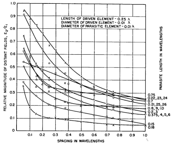
in which k is the complex ratio of I₂/I₁. In such a case, with but one parasitic element, the system is determinate and can be computed from known self- and mutual impedances. With more than one parasitic element, the system is indeterminate because there is insufficient information for a complete solution (see Figs. 3.63A. and 3.63B). Systems using two or more parasitic elements are empirical and must be designed experimentally, though some success by computation can be obtained in simple systems by the method of successive approximations.

FIG. 3.63A. Relative magnitudes of distant fields E2/E1 for driven quarter-wave miipole and parasitic unipoles of different lengths and spacings. (After Abbott and Fisher.)

The block of simultaneous equations applies to any system of radiators having any arbitrary current distributions and any geometrical relationships. The reference points at which the impedances are computed may also be arbitrary. However, the values of self- and mutual impedances will be different in every such case and must usually be computed individually according to the conditions of the case. Equations for most conditions of practical interest have been developed and published for sinusoidal current distributions which are approximated by standing-wave systems. Mutual impedances between radiators carrying traveling waves have to be computed from basic electromagnetic theory.

FIG. 3.63B. Time-phase angle, in degrees, for driven quarter-wave unipole and parasitic unipoles of different lengths and spacings. (After Abbott and Fisher.)