| Radio Antenna Engineering is a free introductory textbook on radio antennas and their applications. See the editorial for more information.... |

|
Home  Impedance-matching Networks Type I Problem Impedance-matching Networks Type I Problem |
||||||||||||||||||||||||||||||||||


|
  |
|||||||||||||||||||||||||||||||||
|
Type I ProblemAuthor: Edmund A. Laport
Problem1: Design a network which will match a 500 ohms resistance load to a 100-ohm source with a phase shift of -30 degrees through the network.
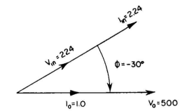
For vector circuit calculations in general, the first step is to set up the original problem in vector form, using convenient scales for potentials and currents and taking the power derived therefrom into consideration. Draw a potential vector and a current vector in phase in a reference direction representing, according to some convenient scale, the 500-ohm load (for example, V0 = 500 volts and I0 = 1 ampere). According to this arbitrarily chosen scale for the vectors, the power W0 represented would be 500 watts. If the impedance-matching network is to have pure reactances, the power input to the network must equal the power represented in the load. The next step is to draw a potential vector and a current vector, in phase, according to the same scale of vectors, which will have a ratio representing the input resistance, a product which gives a power equal to that in the load, and a direction which gives the specified phase shift. Since W0 = 500 watts, and
Figure 5.1 illustrates these first two steps for the problem outlined. This figure represents the problem written vectorially.
We now have a choice of a T or a π solution. Let us choose a T network first and label all the potentials and currents in the load, network, and input in a manner which will satisfy Kirchhoff's laws (see Fig. 5.2). At this point we know V0 and I0, Vin and Iin, R0 and Rin. We represent the network elements as X's because we do not know what is required yet. We also know, from elementary alternating-current theory, that
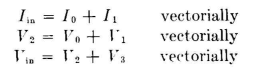
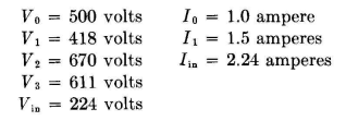
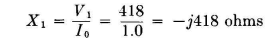
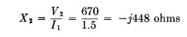
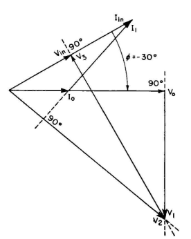
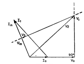
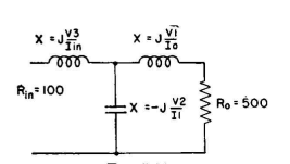
Similarly, we know that for circuit elements which are purely reactive, V1 is perpendicular to I0, V3 is perpendicular to Iin, and V2 is perpendicular to I1. These facts give us enough information to complete the vector diagram for the entire network. This vector diagram has all the information necessary to reveal the nature and magnitude of X1, X2, and X3. There are only three currents in the circuit, and at the outset of the problem we already know two of them. The unknown current I1 can be drawn immediately by connecting the tips of I0 and Iin. The direction of I1 is that which, when added to I0, gives a vector sum Iin. Thus, I1 is directed toward Iin. Its magnitude is determined by its length according to the scale for the current vectors. The intersection of perpendiculars through V0 and Vin locates V2, as shown in Fig. 5.3. The directions are found from considering that V0 + V1 = V2 vectorially and Vin = V2 + V3 vectorially. From the scales for the diagram
where V1 lags I0 by 90 degrees,
where V2 lags I1 by 90 degrees, and
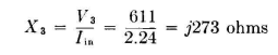
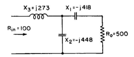
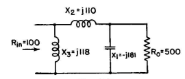
where V3 leads Iin by 90 degrees. The network becomes that shown in Fig. 5.4. A check on the accuracy of construction is offered by the angle between I1 and V2 vectors, which should be 90 degrees. The problem specified a phase difference between V0 and Vin. A different solution results from each different value of phase shift through the network. If phase shift is immaterial, we can find a solution where X1 = 0 and the circuit is simplified to two reactive elements. This is the case where V3 passes through V0 and V1 vanishes; also V2 = V0. The phase shift θ becomes cos-1 (Vin/V0). For values of φ greater than the value where X1 = 0, the sign of X1 changes from -j to +j.2
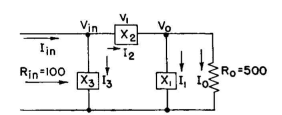
When φ is positive instead of negative, the signs of all the elements reverse likewise. Taking now the π-network solution for the same problem, the circuit becomes that shown in Fig. 5.5. In this case, we know V0, I0, Vin, Iin and φ. We also know X1, X2 and X3 to be pure reactances. Therefore
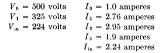
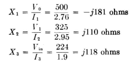
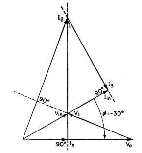
I1 must be perpendicular to V0, I2 must be perpendicular to V1, and I3 must be perpendicular to Vin. Since we know V0 and Vin, we can draw V1 immediately, as shown in Fig. 5.6. From the scales of the diagram
The network becomes that shown in Fig. 5.7.
If the value of φ is immaterial, there is a value at which I3 = 0 and X3 =
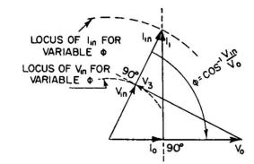
To demonstrate the solution for the two-element circuit to obtain this transformation, we set up input and output vectors but do not specify a phase shift. Instead we allow the input vectors to assume a position which, in the T case, causes V3 to pass directly through V0 and, in the π case, causes I1 to pass through Iin. For example in the π case we draw-the loci of Vin and Iin for variable φ, as shown in Fig. 5.8. Then we erect I1 perpendicular to V0 through I0. Where this cuts the locus of Iin locates the vector Iin.
In the case of the T, X1 becomes 0, and in the case of the π, X3 becomes
Where φ is larger, for the T case, the diagram becomes that shown in
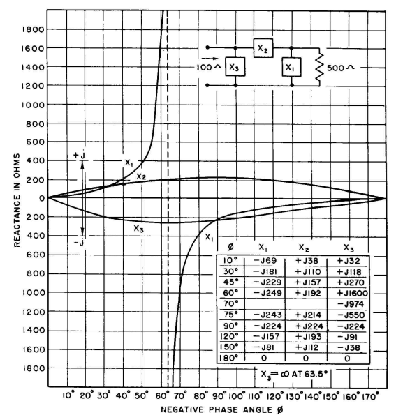
Fig. 5.10. The circuit becomes that shown in Fig. 5.11. Complete curves of reactances for both π and T networks for this transformation as a function of φ are reproduced in Figs. 5.12 and 5.13 to show the nature of the variations. Any impedance-matching problem can be reduced to a type I problem by correcting the power factor of the load or of the generator, when they are other than resistive. This can always be done in either of two ways -by adding series reactance or by adding parallel reactance.
The choice depends upon the relative physical convenience of the ohmic values obtained, whether the desired phase difference is between the currents or the potentials, and the cost or convenience of obtaining the proper reactive components. If a T network is to be used, series power-factor correction of the load impedance or the generator impedance has the advantage that the power-factor-correcting reactors can be combined in value with those found to be necessary from the design synthesis, so that fewer components are ultimately required - three instead of four or five. In the same sense, if a π network is chosen, the parallel method of power-factor correction permits the use of three reactive components instead of four or five by combining the power-factor-correcting reactances with those derived from the network synthesis.
This is virtually what is done in the type II problems. In general, it is always wise to employ network designs requiring the least possible energy storage - that is, the least number of total volt-amperes in all the reactive components. This not only economizes the ratings of the individual components but minimizes the selectivity of the network.This has special importance whenever the bandwidth to be transmitted exceeds 1 percent. The various individual reactances for a network can be made up of lumped capacitance or inductance; or equivalent values of transmission-line sections may be used at frequencies where line sections are preferable.
|
||||||||||||||||||||||||||||||||||
| Home Impedance-matching Networks Type I Problem |
|
|||||||||||||||||||||||||||||||||


 . This particular solution simplifies the circuit to two reactive elements. For values of φ greater than this particular value, the sign of X3 reverses.


Last Update: 2011-03-19