You are working with the text-only light edition of "H.Lohninger: Teach/Me Data Analysis, Springer-Verlag, Berlin-New York-Tokyo, 1999. ISBN 3-540-14743-8". Click here for further information.

Table of Contents Bivariate Data Smoothing Savitzky-Golay Filter - Mathematical Details	Index
See also: filters, Savitzky-Golay filter, coefficients, mathematical background of filters

Savitzky-Golay Filter
Mathematical Details

= Xb = X(X^TX)^-1X^Ty = Hy.

The product H = X(X^TX)^-1X^Ty is also called the hat matrix and is the same for any y for a given polynomial. So it can be calculated once and stored for latter application. This is what Savitzky and Golay have done for polynomials of various orders, and pieces of different length n (original publication and corrections ).

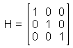
Note: The (n+1)^th row of the H matrix gives the tabulated coefficients for the Savitzky-Golay filters. We only use the estimate for the middle point of the moving window for smoothing. The other rows are used only for the smoothing of the endpoint of the signal, when there are fewer data points left than the window size 2n+1.

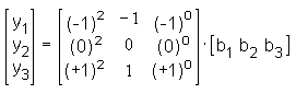
The matrix X is the so-called Vandermond matrix. When we want to fit a polynomial function of order p, we get a series of equations in the following form:

In the case of n=1, x = [-1 0 +1] and we have:

resulting in the filtering coefficients b = [0 1 0]. In this case, actually no calculations would be performed, but rather the original values would be taken. For n=5 and p=3, the filtering coefficients are b= [-0.0857 0.3429 0.4857 0.3429 -0.0857].

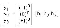
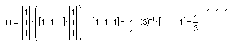
As a special case, we can also derive the moving average, i.e. when we want to fit a constant line (a zero^th order polynomial).
 

Last Update: 2006-Jän-17