Propagation Constant and Characteristic Impedance of a Cable

Approximate Propagation Constant of a Cable. The general expression for the propagation constant is given by equation 36 as

γ = sqrt((R +jX)(G +jB)). When the substitutions X = ωL and B = ωC are made and L and G are assumed to be zero, then

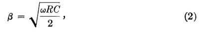
From this equation, or from equations 48 and 49 when L and G are assumed zero.

and

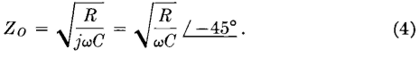
where β will be in radians per mile and a will be in nepers per mile when R is in ohms per loop mile, C is in farads per mile of cable, and ω is 2π times the frequency in cycles per second.

Approximate Characteristic Impedance of a Cable. The characteristic impedance of any two-wire transmission circuit is given by equation 50 as Z_o = sqrt((R + jωL)/(G +jωC)). If L and G are negligible,

The magnitude of the characteristic impedance will be in ohms when R is in ohms, C is in farads, and ω is 2π times the frequency in cycles per second. The values of R and C can be for any lengths, provided that they are the same. Since the characteristic impedance of a circuit determines the magnitude and phase angle of the current, it is important to note that from equation 4 the current at each point along a cable will lead the voltage at that point by 45°. This assumes, of course, that the cable is terminated in its characteristic impedance.

Actual values of β, α, and Z₀ will be found in Table I, page 250, Table III, page 253, and the high-frequency loss in decibels in Fig. 6. Additional data at high frequencies are given in reference 4.