Algebraical Approximation

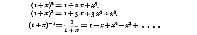
If we only require to use a formula to give a result accurate within certain limits, it is, in many cases, possible to save a large amount of arithmetical labour by altering the form of the formula to be employed. This is most frequently the case when any small correction to the value of one of the observed elements has to be introduced, as in the case, for instance, of an observed barometric height which has to be corrected for temperature. We substitute for the strictly accurate formula an approximate one, which renders the calculation easier, but in the end gives the same result to the required degree of accuracy.

We have already said that an accuracy of one part in a thousand is, as a rule, ample for our purpose; and we may, therefore, for the sake of definiteness, consider the simplification of algebraical formulae with the specification of one part in a thousand, or 0.1 percent, as the limit of accuracy desired. Whatever we have to say may be easily adapted for a higher degree of accuracy, if such be found to be necessary.

It is shown in works on algebra that

This is known as the 'binomial theorem,' and is true for all values of n positive or negative, integral or fractional. Some special cases will probably be familiar to every student, as:

If we change the sign of x we get the general formula in the form

We may include both in one form, thus:

where the sign +/- means that either the + or the - is to be taken throughout.

Now, if x be a small fraction, say, 1/1000 or 0.001, x² is evidently a much smaller fraction, namely, 1/1000000, or 0.000001, and x³ is still smaller. Thus, unless n is very large indeed, the term

will be too small to be taken account of, and the terms which follow will be of still less importance. We shall probably not meet with formulae in which n is greater than 3. Let us then determine the value of x so that

may be equal to 0.001, that is to say, may just make itself felt in the calculations that we are now discussing. Putting n = 3 we get

So that we shall be well within the truth if we say that (when n = 3), if x be not greater than 0.01, the third term of equation (1) is less than 0.001, and the fourth term less than 0.00001. Neither of these, nor anyone beyond them, will, therefore, affect the result, as far as an accuracy of one part in a thousand is concerned; and we may, therefore, say that, if x is not greater than 0.01,

To use this approximate formula when x = 0.01 would be inadmissible, as it produces a considerable effect upon the next decimal place; and, if in the same formula, we make other approximations of a similar nature, the accumulation of approximation may impair the accuracy of the result.

In any special case, therefore, it is well to consider whether x is small enough to allow of the use of the approximate formula by roughly calculating the value of the third term; it is nearly always so if it is less than 0.005. This includes the important case in which x is the coefficient of expansion of a gas for which x = 0.00366.

If n be smaller than 3, what we have said is true within still closer limits; and as n is usually smaller than 3, we may say generally that, for our purposes,

and

provided x be less than 0.005.

Some special cases of the application of this method of approximation are here given, as they are of frequent occurrence:

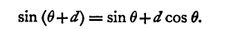
The formulae for +x and -x are here included in one expression; the upper or lower sign must be taken throughout the formula.

We thus see that whenever a factor of the form (1±x)ⁿ occurs in a formula where x is a small fraction, we may replace it by the simpler but approximate factor 1±nx; and we have already shown how the multiplication by such a factor may be very simply performed (p. 39). Cases of the application of this method occur in §§13, 24 etc.

Another instance of the change of formula for the purposes of arithmetical simplicity is made use of in §13. In that case we obtain a result as the geometric mean of two nearly equal quantities. It is an easy matter to prove algebraically, although we have not space to give the proof here, that the geometric mean of two quantities which differ pnly by one part in a thousand differs from the arithmetic mean, of the two quantities by less than the millionth of either. It is a much easier arithmetical operation to find the arithmetic mean than the geometric, so that we substitute in the formula (x+x')/2 for sqrt(x x').

The calculation of the effect upon the trigonometrical ratios of an angle, due to a small fractional increase in the angle, may be included in this section. We know that

Now, reference to a table of sines and cosines will show that cos d differs from unity by less than one part in a thousand if d be less than 2° 33', and, if expressed in circular measure, the same value of d differs from sin d by one part in three thousand; so we may say that, provided d is less than 2.5°, cos d is equal to unity, and sin d is equal to d expressed in circular measure.

The formula is, therefore, for our purposes, equivalent to

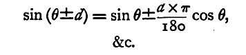
We may reason about the other trigonometrical ratios in a similar manner, and we thus get the following approximate formulae:

The upper or lower sign is to be taken throughout the formula.

If d be expressed in degrees, then, since the circular measure of 1° is π/180, that of d° is dπ/180, and the formulae become

It has been already stated that approximate formulas are frequently available when it is required to introduce corrections for variations of temperature, and other elements which may be taken from tables of constants. There is besides another use for them which should not be overlooked, namely, to calculate the effect upon the result of an error of given magnitude in one of the observed elements. This is practically the same as calculating the effect of a hypothetical correction to one of the observed elements. In cases where the formula of reduction is simply the product or quotient of a number of factors each of which is observed directly, a fractional error of any magnitude in one of the factors produces in the result an error of the same fractional magnitude, but in other cases the effect is not so simply calculated. If we take one example it will serve to illustrate our meaning, and the general method of employing the approximate formulae we have given in this chapter.

In §75 electric currents are measured by the tangent galvanometer. Suppose that in reading the galvanometer we cannot be sure of the position of the needle to a greater accuracy than a quarter of a degree. Let us, therefore, consider the following question: 'To find the effect upon the value of a current, as deduced from observations with the tangent galvanometer, of an error of a quarter of a degree in the reading?'

The formula of reduction is

Suppose an error δ has been made in the reading of θ, so that the observed value is

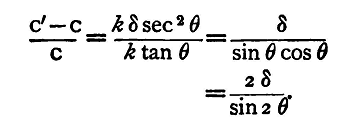
The fractional error q in the result is

The error δ must be expressed in circular measure; if it be equivalent to a quarter of a degree, we have

The actual magnitude of this fraction depends upon the value of θ, that is upon the deflection. It is evidently very great when θ is very small, and least when θ = 45°, when it is 0.9 percent. From which we see not only that when θ is known the effect of the error can be calculated, but also that the effect of an error of reading, of given magnitude, is least when the deflection is 45°. It is clear from this that a tangent galvanometer reading is most accurate when the deflection produced by the current is 45°. This furnishes an instance, therefore, of the manner in which the approximate formulae we have given in this chapter can be used to determine what is the best experimental arrangement of the magnitudes of the quantities employed, for securing the greatest accuracy in an experiment with given apparatus. The same plan may be adopted to calculate the best arrangement of the apparatus for any of the experiments described below.

In concluding this part of the subject, we wish to draw special attention to one or two cases, already hinted at, in which either the method of making the experiments, or the formula for reduction, makes it necessary to pay special attention to the accuracy of some of the elements observed. In illustration of the former case we may mention the weighing of a small mass contained in a large vessel. To fix ideas on the subject, consider the determination of the mass of a given volume of gas contained in a glass globe, by weighing the globe full and empty. During the interval between the two weighings the temperature and pressure of the air, and in consequence the apparent weight of the glass vessel, may have altered. This change, unless allowed for, will appear, when the subtraction has been performed, as an error of the same actual magnitude in the mass of the gas, and may be a very large fraction of the observed mass of the gas, so that we must here take account of the variation in the correction for weighing in air, although such a precaution might be quite unnecessary if we simply wished to determine the actual mass of the glass vessel and its contents to the degree of accuracy that we have hitherto assumed. A case of the same kind occurs in the determination ot the quantity of moisture in the air by means of drying tubes (§42).

Cases of the second kind referred to above often arise from the fact that the formulae contain differences of nearly equal quantities; we may refer to the formulas employed in the correction of the first observations with Atwood's machine, the determination of the latent heat of steam, and the determination of the focal length of a concave lens (§54) as instances. In illustration of this point we may give the following question, in which the hypothetical errors introduced are not really very exaggerated.

'An observer, in making experiments to determine the focal length of a concave lens, measures the focal length of the auxiliary lens as 10.5 cm., when it is really 10 cm., and the focal length of the combination as 14.5 cm., when it is really 15 cm.; find the error in the result introduced by the inaccuracies in the measurements.'

We have the formula

whence

putting in the true values of F and f₁.

and putting the observed values

The fractional error thus introduced is

or more than 25 percent, whereas the error in either observation was not greater than 5 percent.

It will be seen that the large increase in the percentage error is due to the fact that the difference in the errors in F and f₁ has to be estimated as a fraction of F-f₁; this should lead us to select such a value of f₁ as will make F-f₁ as great as possible, in order that errors of given actual magnitude in the observations may produce in the result a fractional error as small as possible.

We have not space for more detail on this subject. The student will, we hope, be able to understand from the instances given that a large amount of valuable information as to the suitability of particular methods, and the selectior of proper apparatus for making certain measurements, can be obtained from a consideration of the formulae of reduction in the manner we have here briefly indicated.