You are working with the text-only light edition of "H.Lohninger: Teach/Me Data Analysis, Springer-Verlag, Berlin-New York-Tokyo, 1999. ISBN 3-540-14743-8". Click here for further information.

Table of Contents Univariate Data Distributions Introduction	Index
See also: variability, Fractiles, Central Limit Theorem

Distributions
Introduction Part 1

If you take subsequent samples from the same random process you will get different results. The mean of these results and its spread are usually a good indicator of the process being sampled. A short example should clarify this:

Assume a physicist is baking a plum cake, and puts exactly 75 plums into the dough. After stirring the dough and baking the cake, he cuts a piece of the cake, which is exactly one third of its size. As this physicist has enough spare time, he crumbles this slice and counts the plums in it - only 19 of the expected 25 plums are found. Now the question which keeps the physicist from finally eating the cake is how are the chances of getting a slice of this size with less than 20 plums in it?

Before looking into a statistics textbook you may want to perform an experiment yourself. Click on the to start the experiment !

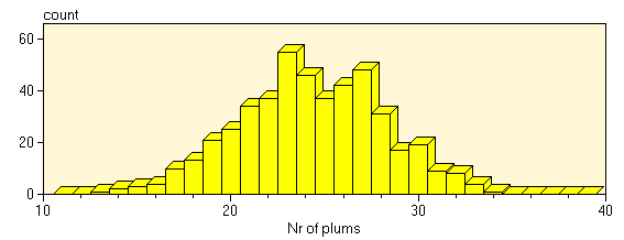
What you see is, that the actual number of plums in a third of the cake varies around 25. The histogram of the frequency of occurrence of different numbers of plums may look like this:

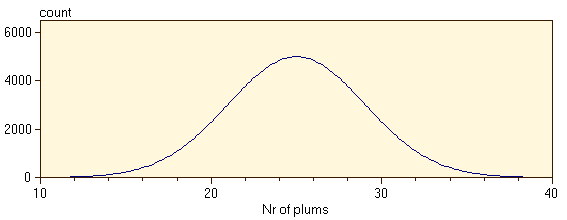
If you repeat the process of plum cake baking often enough, and you plot the histogram bars small enough you will eventually obtain a smooth distribution:

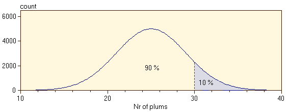
Next, our physicist wants to know how what the chances are of finding more than 30 plums in the slice of the plum cake. One of the fundamental properties of distribution diagrams is that the relative area between two values on the x-axis reflect the chances that the corresponding event will occur. In our example the physicist may draw a vertical line at 30 plums. The relative area above this mark indicates the chance of finding more than 30 plums in the slice of cake (which is roughly 10 %, according to the distribution curve shown below).
 

Sometimes it may be inconvenient to determine the relative area. This complication can be avoided by scaling the distribution curve such that it has an area of exactly 1.0. When doing so, any area below the curve reflects the chances that an event may fall into that area. This curve is called the probability density function (pdf):

Hint:    Do not confuse the scaling of the area with the scaling of the y-axis. A distribution curve scaled to an area of 1.0 does not have a maximum of 1.0; see also the for further explanation

Last Update: 2006-Jän-17