| Electrical Communication is a free textbook on the basics of communication technology. See the editorial for more information.... |

|
Home  Electric Networks Filters Low-Pass Filter Electric Networks Filters Low-Pass Filter |
|||||||||||


|
  |
||||||||||
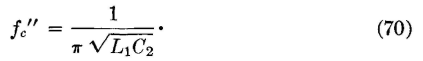
Low-Pass FilterA properly terminated low-pass filter with no power losses in the elements will pass, without attenuation, signals of all frequencies from zero up to a critical cutoff frequency, and will attenuate signals above this frequency. Three sections of a low-pass filter are shown in Fig. 27. These will pass signals of such frequencies that Z1/Z2 lies between 0 and -4. In Fig. 27 the series impedances are Z1 = jωL1 and the shunt impedances are Z2 = l/(jωC2). Then, Z1/Z2 = (jωL1)(jωC2) = -ω2L1C2. When Z1/Z2 = 0, the lower cutoff frequency is found; thus, since ω = 2πf, Z1/Z2 = -ωc2L1C2 = -(2πfc')2L1C2 = 0, and fc' = 0. When Z1/Z2 = -ωC2L1C2 = -(2πfc")2L1C2 = -4, then the upper cutoff frequency is
The low-pass filter will accordingly pass currents of all frequencies from direct current (f = 0) up to the value given by equation 70. The variations of the iterative impedances of T and π low-pass filter sections will now be investigated. From equation 45,
when -ωc2L1C2 = -4 and ωc" = 2πfc" are substituted. This equation gives the iterative impedance of the low-pass T section of Fig. 27 at any given frequency ratio f/fc". By a similar process it can be shown that, for the π section, equation 46 becomes
The equations for these two impedance curves are shown plotted in Fig. 28. They show that, for f = 0,
for both the T and the π sections. They further show that the impedance values then diverge and that at the value f = fc" (that is, at the cutoff frequency) ZKT = 0 and Z Kπ = ∞. It is common practice to design a low-pass filter so that the iterative impedance ZK computed at f = 0 and given by equation 73 equals the impedance of the line in which it is to operate. It is now possible to derive the design equations for low-pass filters. The upper cutoff frequency was found from the relation -ωc2L1C2 = -4. If 2πfc" is substituted for ωc, this relation can be arranged L1/C2 = (2πfc"L1)2/4. But ZK = sqrt(L1/C2), and thus
Therefore,
Using these two equations, simple low-pass constant-k filters can be designed as will be illustrated. Suppose that it is desired to construct a low-pass filter having an iterative impedance of 600 ohms and a cutoff frequency of 1000 cycles. From equation 74, L1 = 600/(3.1416 x 1000) = 0.191 henry, and from equation 75, C2 = 1/(3.1416 x 1000 x 600) = 0.000000530 farad or 0.53 microfarad. That is, the series element Z1 of Fig. 27 must be 0.191 henry inductance and the shunt element Z2 of Fig. 27 must be 0.53 microfarad capacitance.
The filter section can be connected either as a T or as a π section. If connected as a T section, two inductors each having an inductance of 0.191/2 or 0.0955 henry, and one capacitor having a capacitance of 0.53 microfarad, will be required. If connected as a π section, one 0.191-henry inductor and two 0.53/2 = 0.265-microfarad capacitors will be needed. These relations will be evident from Figs. 4, 5, and 6. It should also be noted that
Of particular interest in filter studies are the iterative impedance that has been considered, and the attenuation and phase shift that will now be treated. If the filter elements are pure reactances, the attenuation will be zero for frequencies within the band passed and will be as given by equation 67 for frequencies beyond the band passed. For the low-pass filter of Fig. 27,
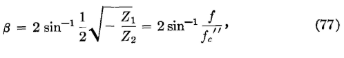
when the value given by equation 74 is substituted for L1, and the value given by equation 75 is substituted for C2. Thus, at 2000 cycles the attenuation of the low-pass filter under consideration will be α = 2 cosh-1 (2000/1000) = 2 cosh-1 2, and α = 2 x 1.31 = 2.62 nepers, the value 1.31 being determined from a table of hyperbolic functions. The corresponding loss in decibels is db = 2.62 x 8.686 = 22.8 decibels. The dotted curve of Fig. 29 was computed in this way. The solid curve of Fig. 29 was measured on an actual filter section, the elements of which had some loss. For methods of calculating the attenuation in which the losses of the filter elements are considered, reference 4 should be consulted. If the elements of a low-pass filter are pure reactances, there will be a varying phase shift over the band passed, and a constant phase shift of 180° beyond the band passed. From equation 63, and for the low-pass filter,
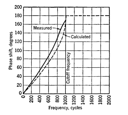
when the substitutions as in equation 76 are made. Thus, for the low-pass filter under consideration, and at 500 cycles, β = 2 sin-1 (500/1000) = 2 sin-1 0.5 = 60°. The dotted curve of Fig. 30 was
computed in this manner, and the solid curve was measured on an actual filter section, the elements of which had some loss. The phase measurements were made with a cathode-ray oscilloscope.
The transmission and attenuation bands of low-pass filters can be determined from simple reactance sketches as in Fig. 31. Thus, if curves for Z1 (equals 2πL1) and -4Z2 (where Z2 = l/(2πf/C2)) are plotted as indicated, the transmission band T will occur where Z1 lies between the frequency axis and the curve -4Z2, and the band A where Z1 lies without curve -4Z2 will be attenuated.
|
|||||||||||
| Home Electric Networks Filters Low-Pass Filter |
|
||||||||||


Last Update: 2011-06-05